Feature Selection in World Models: A Spectral View
Which features do world-model objectives preserve for planning, and which do they discard? A first-principles comparison of five objectives in a shared linear-Gaussian setting.
Which features do world-model objectives preserve for planning, and which do they discard?
World models compress observations into latent states that an agent can use to predict how the world will evolve under different actions and plan accordingly. This compression makes planning tractable, but it also forces a choice: which features remain available to the planner, and which are discarded?
In this post, we compare five world-model objectives from first principles. Placing all five in the same linear-Gaussian setting, with data collected under a purely exploratory policy, we find that each yields a simple score that determines which modes enter the representation. The scores reveal a spectrum: VAE-based World Models
Model Predictive Control with Linear Dynamics
We consider a model predictive control (MPC) setup in which the world model extracts features from raw observations and predicts how these latent features evolve under different actions. The choice of features is crucial for the downstream task, since it determines what information the planner can use.
To make the analysis tractable, we consider linear dynamics with Gaussian process noise and quadratic control costs, a classical setting for MPC
The system evolves as
\[\begin{aligned} \mathbf X_{t+1} &=\mathbf A_{\mathrm X}\mathbf X_t +\mathbf B_{\mathrm X}\mathbf U_t+\boldsymbol\varepsilon_t,\\ \boldsymbol\varepsilon_t&\sim\mathcal N(\mathbf 0,\mathbf Q). \end{aligned}\]Here \(\mathbf X_t\) is the observed state, \(\mathbf U_t\) is the action, and \(\boldsymbol\varepsilon_t\) is fresh process noise. We assume stable dynamics and a stationary, centered state distribution. During data collection, actions are sampled from a purely exploratory Gaussian policy, independently of the state and noise; this is distinct from the control policy later optimized by the planner.
Our goal is to understand which directions of variation in \(\mathbf X_t\) each world-model objective chooses to preserve. To obtain a simple closed-form comparison, we assume that the dynamics, state covariance, action-induced covariance, and noise covariance share an orthonormal basis \(\{\boldsymbol\phi_j\}_{j=1}^d\). We refer to these directions as modes.
Write \(\boldsymbol\Sigma_{\mathrm X}=\operatorname{Cov}(\mathbf X_t)\) for the state covariance and \(\boldsymbol\Sigma_{\mathrm U}=\operatorname{Cov}(\mathbf U_t)\) for the action covariance. Each mode \(j\) is characterized by
\[\boldsymbol\Sigma_{\mathrm X}\boldsymbol\phi_j=p_j\boldsymbol\phi_j, \qquad \mathbf A_{\mathrm X}\boldsymbol\phi_j=\rho_j\boldsymbol\phi_j, \qquad \boldsymbol\phi_j^\top\mathbf B_{\mathrm X} \boldsymbol\Sigma_{\mathrm U}\mathbf B_{\mathrm X}^\top \boldsymbol\phi_j=p_jc_j.\]The quantity \(p_j\) measures how much the observations vary along mode \(j\). The fraction \(\rho_j^2\) measures how much of its next-step variance is predictable from the current state, while \(c_j\) measures the fraction predictable from the action. We write
\[a_j=\rho_j^2+c_j\]for the total predictable fraction of the mode. Stationarity then gives \(\boldsymbol\phi_j^\top\mathbf Q\boldsymbol\phi_j=p_j(1-a_j)\), so \(1-a_j\) is the fraction of the mode generated by fresh, unpredictable noise.
Each mode is summarized by two main quantities
- \(p_j\) (observation variance): how much the mode varies.
- \(a_j\) (predictable fraction): how much of its next-step variance can be predicted from the current state and action.
The different world-model objectives we study rank these same modes differently. To make this comparison explicit, we derive a mode-selection score for each objective. When the representation is limited to \(k\) features, modes with higher scores are selected first. What changes across objectives is how that score is defined: some depend only on observation variance, some only on predictability, and others trade off the two.
This spectral perspective is also related to Koopman-based control, where nonlinear dynamics are approximated by linear prediction in a learned feature space
In this setting, each objective has a simple mode-selection rule. The table below summarizes them, and the rest of this section derives each one.
| Objective | Mode-selection rule | Interpretation |
|---|---|---|
| VAE | \(p_j\) | variance only |
| Observation prediction | \(p_j a_j\) | variance and predictability |
| E2C | \(p_j(1+a_j)\), plus a predictability bonus | variance, amplified by predictability |
| Dreamer | \(p_j\), plus a predictability bonus | variance or predictability can compensate |
| JEPA | \(a_j\) | predictability only |
VAE World Models: Reconstruct First, Predict Later
We start our exploration with the seminal work of Ha and Schmidhuber
We use a deterministic approximation for variational methods: we replace sampled latents with their encoder means, fix the covariance terms, and retain only the mean-dependent parts of the loss. This results in squared reconstruction and prediction errors, which are sufficient to illustrate the competition between features studied in this blog. The dropdowns provide the corresponding probabilistic objectives and explain the terms omitted by our approximation.
Throughout the five simplified objectives, \(\mathbf E\) denotes the encoder parameters, \(\mathbf D\) the decoder parameters, and \(\mathbf P\) the action-conditioned predictor parameters. We optimize the parameters listed under each minimum; the data distribution, latent capacity, loss weights, and covariance scales are held fixed. The linear mode-selection results additionally impose the normalization and model restrictions stated in the proofs.
To understand which features the VAE stage retains, let \(\mathbf X_t\in\mathbb R^d\) be a centered observation with covariance \(\boldsymbol\Sigma_{\mathrm X}\succ0\). The encoder maps \(\mathbf X_t\) to its latent representation \(\mathbf Z_t=f_{\mathbf E}^{\mathrm{enc}}(\mathbf X_t)\), while the decoder \(f_{\mathbf D}^{\mathrm{dec}}(\mathbf Z_t)\) reconstructs the original observation. With decoder variance \(\sigma_{\mathrm{dec}}^2>0\) and regularization weight \(\beta>0\), the simplified mean objective is
The variational VAE loss and our approximation
The VAE stage of World Models combines reconstruction with a KL penalty toward a standard Gaussian prior
For a Gaussian encoder \(q_{\mathbf E}=\mathcal N(\boldsymbol\mu,\mathbf C)\), where \(\boldsymbol\mu=f_{\mathbf E}^{\mathrm{enc}}(\mathbf X_t)\), the KL is
\[\frac12\left[ \|\boldsymbol\mu\|_2^2+\operatorname{tr}(\mathbf C) -\log\det\mathbf C-k\right].\]A fixed-variance Gaussian decoder gives a squared reconstruction loss. Our approximation evaluates the decoder at \(\boldsymbol\mu\) and keeps the quadratic mean term of the KL. It omits covariance learning and the effect of posterior sampling on reconstruction. For example, with a linear decoder, sampling contributes the additional term \(\operatorname{tr}(\mathbf D\mathbf C\mathbf D^\top)/(2\sigma_{\mathrm{dec}}^2)\), which depends on the decoder even when \(\mathbf C\) is fixed. The normalization used for our feature-selection result is a further assumption, stated in the proof below.
In the World Models paper, the authors then train a recurrent latent predictor while keeping the encoder fixed.
The first term rewards reconstruction. The second is the encoder-mean contribution of the VAE’s KL penalty. For the linear analysis, we normalize the active latent coordinates; this makes the second term cost \(\beta/2\) per active feature and prevents arbitrary rescaling of the encoder and decoder. The precise constraint is given in the proof below.
Under the spectral setup introduced above, the solution keeps up to \(k\) modes with the largest positive scores
The interpretation is simple: apart from the shared offset \(\beta\), the VAE scores and ranks modes only by their observation variance \(p_j\). Neither their predictability \(a_j\) nor the extent to which they are influenced by actions enters the score. The VAE preserves what varies most in the observations, regardless of whether that variation is predictable.
Derivation of the VAE mode-selection score
Assumptions. All five derivations concern the simplified linear objectives above, with observation variances \(p_j>0\), an integer capacity \(1\leq k\leq d\), and predictable fractions \(0\leq a_j\leq1\) as implied by stationarity. The later proofs add their own restrictions without repeating these.
Let \(\boldsymbol\Sigma_{\mathrm X}\succ0\) be the observation covariance, with orthonormal eigenvectors \(\boldsymbol\phi_j\) and eigenvalues \(p_j\):
\[\boldsymbol\Sigma_{\mathrm X}\boldsymbol\phi_j =p_j\boldsymbol\phi_j.\]Linear specialization. Let \(\mathbf E\in\mathbb R^{r\times d}\) and \(\mathbf D\in\mathbb R^{d\times r}\) be the encoder and decoder matrices:
\[\mathbf Z_t=\mathbf E\mathbf X_t, \qquad \widehat{\mathbf X}_t=\mathbf D\mathbf Z_t, \qquad \mathbf E\boldsymbol\Sigma_{\mathrm X}\mathbf E^\top=\mathbf I_r, \qquad 0\leq r\leq k.\]The normalization fixes the scale of every active coordinate. In particular,
\[\mathbb E\|\mathbf E\mathbf X_t\|_2^2 =\operatorname{tr}(\mathbf E\boldsymbol\Sigma_{\mathrm X}\mathbf E^\top) =r,\]so the mean-dependent KL contribution is \(\beta r/2\).
Optimal decoder. For a fixed normalized encoder, completing the square gives
\[\begin{aligned} \mathbb E\|\mathbf D\mathbf E\mathbf X_t-\mathbf X_t\|_2^2 ={}&\operatorname{tr}(\boldsymbol\Sigma_{\mathrm X}) -\operatorname{tr}(\mathbf E\boldsymbol\Sigma_{\mathrm X}^2\mathbf E^\top)\\ &+\|\mathbf D-\boldsymbol\Sigma_{\mathrm X}\mathbf E^\top\|_F^2. \end{aligned}\]The final term is minimized at
\[\mathbf D^\star=\boldsymbol\Sigma_{\mathrm X}\mathbf E^\top.\]Define the whitened encoder
\[\mathbf W:=\mathbf E\boldsymbol\Sigma_{\mathrm X}^{1/2}.\]Then \(\mathbf W\mathbf W^\top=\mathbf I_r\). The matrix
\[\boldsymbol\Pi:=\mathbf W^\top\mathbf W\]is therefore the orthogonal projector onto the row space of the whitened encoder \(\mathbf W\):
\[\boldsymbol\Pi^2=\boldsymbol\Pi, \qquad \boldsymbol\Pi^\top=\boldsymbol\Pi, \qquad \operatorname{tr}(\boldsymbol\Pi)=r\leq k.\]Using cyclicity of the trace,
\[\operatorname{tr}(\mathbf E\boldsymbol\Sigma_{\mathrm X}^2\mathbf E^\top) =\operatorname{tr}(\boldsymbol\Pi\boldsymbol\Sigma_{\mathrm X}).\]Conversely, every rank-\(r\) orthogonal projector can be written as \(\mathbf W^\top\mathbf W\) by taking the rows of \(\mathbf W\) to be an orthonormal basis of its range. Setting \(\mathbf E=\mathbf W\boldsymbol\Sigma_{\mathrm X}^{-1/2}\) then gives an admissible normalized encoder. Thus this change of variables loses no admissible encoder subspaces.
After optimizing the decoder, the VAE loss is consequently
\[\mathcal L_{\mathrm{VAE}}^\star(\boldsymbol\Pi) =\frac{\operatorname{tr}(\boldsymbol\Sigma_{\mathrm X})} {2\sigma_{\mathrm{dec}}^2} -\frac12\operatorname{tr} \left[ \boldsymbol\Pi \left( \frac{\boldsymbol\Sigma_{\mathrm X}}{\sigma_{\mathrm{dec}}^2} -\beta\mathbf I_d \right) \right].\]Optimal encoder directions. Define the symmetric score matrix
\[\mathbf H_{\mathrm{VAE}} :=\frac{\boldsymbol\Sigma_{\mathrm X}}{\sigma_{\mathrm{dec}}^2} -\beta\mathbf I_d.\]Its eigenvectors are the observation covariance eigenvectors \(\boldsymbol\phi_j\), with eigenvalues
\[h_j:=\frac{p_j}{\sigma_{\mathrm{dec}}^2}-\beta.\]Minimizing the loss is therefore equivalent to maximizing \(\operatorname{tr}(\boldsymbol\Pi\mathbf H_{\mathrm{VAE}})\) over encoder subspaces of dimension at most \(k\). Expand this trace in the eigenbasis:
\[\operatorname{tr}(\boldsymbol\Pi\mathbf H_{\mathrm{VAE}}) =\sum_{j=1}^d h_jq_j, \qquad q_j:=\boldsymbol\phi_j^\top\boldsymbol\Pi\boldsymbol\phi_j =\|\boldsymbol\Pi\boldsymbol\phi_j\|_2^2.\]Here \(q_j\) is the squared length of mode \(j\)’s projection onto the encoder subspace. Because \(\boldsymbol\Pi\) is an orthogonal projector,
\[0\leq q_j\leq1, \qquad \sum_jq_j=\operatorname{tr}(\boldsymbol\Pi)\leq k.\]The weighted sum cannot exceed the sum of the \(k\) largest positive \(h_j\) (or all positive \(h_j\) if there are fewer than \(k\)). This bound is attained by projecting onto exactly those modes:
\[\boldsymbol\Pi^\star =\sum_{j\in S}\boldsymbol\phi_j\boldsymbol\phi_j^\top,\]where \(S\) indexes the selected modes. Thus a mode-aligned encoder is globally optimal among all normalized linear encoders; its alignment has been derived, rather than assumed.
Recovering the encoder and decoder. For every selected mode \(j\in S\), take
\[\mathbf E_j=\frac{\boldsymbol\phi_j^\top}{\sqrt{p_j}}, \qquad \mathbf D_j^\star=\sqrt{p_j}\boldsymbol\phi_j.\]These rows and columns realize the projector \(\boldsymbol\Pi^\star\) and the optimal decoder derived above.
Mode-selection score. Retaining mode \(j\) decreases the profiled loss by \(h_j/2\). Dropping the common positive factor \(1/2\) gives
\[\boxed{ \operatorname{score}_j^{\mathrm{VAE}} =\frac{p_j}{\sigma_{\mathrm{dec}}^2}-\beta }.\]The closed-form solution selects the largest positive scores, up to capacity \(k\). If every score is nonpositive, the zero representation is optimal; zero-score modes leave the loss unchanged, and ties may be resolved arbitrarily.
Action-Conditioned Observation Prediction: Predict What Comes Next
Instead of learning to reconstruct the current observation, one can train the world model to predict the next observation from the current one and the action. This is the idea behind action-conditioned video prediction
The encoder produces \(\mathbf Z_t=f_{\mathbf E}^{\mathrm{enc}}(\mathbf X_t)\). The predictor combines this representation with the action, and the decoder maps the predicted latent state back to observation space:
The observation-prediction loss and our approximation
Oh et al.
Here \(H\) is the training prediction horizon. The predictions use the observed frame history and the intervening actions; multi-step training feeds predicted frames back into the model. The paper includes both a fixed-history encoder and a recurrent encoder, and increases \(H\) during training.
Our comparison uses \(H=1\), the current observation and action, and a fixed Gaussian likelihood scale. The squared-error learning signal is already present in the original method. The simplification concerns the history, prediction horizon, and linear maps used in the proof.
Unlike the VAE objective, there is no KL penalty charging for each active feature. Instead, a feature is useful only when it helps predict the next observation. Here, the optimal predicted output keeps up to \(k\) modes with the largest scores. Because the action enters the predictor directly, this ranks modes in the predicted output; it does not uniquely determine what the encoder stores.
The contrast with the VAE is immediate: modes are now ranked by predictable variance, \(p_j a_j\), rather than total variance \(p_j\). A high-variance mode that is entirely driven by fresh noise has \(a_j=0\) and provides no benefit.
Observation prediction filters out variation that cannot be predicted, but it still favors large-scale variation in observation space. A large, moderately predictable mode can outrank a small, highly predictable one.
Derivation of the observation-prediction mode-selection score
Use the common eigenbasis from the setup. Thus
\[\boldsymbol\Sigma_{\mathrm X}\boldsymbol\phi_j =p_j\boldsymbol\phi_j,\]and mode \(j\) has predictable fraction \(a_j\).
The predictable part of the next observation. Under squared error, the best unconstrained prediction of \(\mathbf X_{t+1}\) from \((\mathbf X_t,\mathbf U_t)\) is its conditional mean
\[\mathbf M_t :=\mathbb E[\mathbf X_{t+1}\mid\mathbf X_t,\mathbf U_t] =\mathbf A_{\mathrm X}\mathbf X_t+\mathbf B_{\mathrm X}\mathbf U_t.\]Because the process noise is independent of \((\mathbf X_t,\mathbf U_t)\),
\[\mathbf X_{t+1}=\mathbf M_t+\boldsymbol\varepsilon_t.\]The covariance of the predictable part is
\[\begin{aligned} \mathbf C_{\mathrm M} :=\operatorname{Cov}(\mathbf M_t) &=\sum_{j=1}^d p_j(\rho_j^2+c_j) \boldsymbol\phi_j\boldsymbol\phi_j^\top\\ &=\sum_{j=1}^d p_ja_j\boldsymbol\phi_j\boldsymbol\phi_j^\top. \end{aligned}\]Hence the eigenvectors of \(\mathbf C_{\mathrm M}\) are the common modes \(\boldsymbol\phi_j\), and its eigenvalue in mode \(j\) is the predictable observation variance \(p_ja_j\).
From the network to a reduced-rank problem. In the linear specialization,
\[\begin{aligned} \mathbf Z_t&=\mathbf E\mathbf X_t,\\ \widehat{\mathbf Z}_{t+1} &=\mathbf K\mathbf Z_t+\mathbf B\mathbf U_t,\\ \widehat{\mathbf X}_{t+1} &=\mathbf D\widehat{\mathbf Z}_{t+1}, \end{aligned}\]where the number of active coordinates is \(r\leq k\) and \(\mathbf E\boldsymbol\Sigma_{\mathrm X}\mathbf E^\top=\mathbf I_r\). The original optimization over \((\mathbf E,\mathbf K,\mathbf B,\mathbf D)\) is not jointly convex: its prediction contains the products \(\mathbf D\mathbf K\mathbf E\) and \(\mathbf D\mathbf B\). We therefore do not use first-order conditions in the raw network parameters.
Instead, observe that every decoded prediction belongs to the output subspace
\[\mathcal U:=\operatorname{range}(\mathbf D), \qquad \dim(\mathcal U)\leq r\leq k.\]Let \(\boldsymbol\Pi_{\mathcal U}\) be the orthogonal projector onto this subspace. Among all \(\mathcal U\)-valued predictions, the one closest to \(\mathbf M_t\) is its orthogonal projection \(\boldsymbol\Pi_{\mathcal U}\mathbf M_t\). Therefore every network with output subspace \(\mathcal U\) satisfies
\[\begin{aligned} \mathbb E\|\mathbf X_{t+1}-\widehat{\mathbf X}_{t+1}\|_2^2 &\geq \mathbb E\|\mathbf X_{t+1} -\boldsymbol\Pi_{\mathcal U}\mathbf M_t\|_2^2\\ &=\operatorname{tr}(\boldsymbol\Sigma_{\mathrm X}) -\operatorname{tr}(\boldsymbol\Pi_{\mathcal U}\mathbf C_{\mathrm M}). \end{aligned}\]The inequality uses the orthogonal decomposition into fresh noise and conditional-mean prediction error. The equality uses stationarity, \(\boldsymbol\Sigma_{\mathrm X}=\mathbf C_{\mathrm M}+\mathbf Q\).
Optimal output directions. Minimizing the error bound amounts to maximizing the captured predictable variance \(\operatorname{tr}(\boldsymbol\Pi_{\mathcal U}\mathbf C_{\mathrm M})\). Expanding in the eigenbasis of \(\mathbf C_{\mathrm M}\) gives
\[\operatorname{tr}(\boldsymbol\Pi_{\mathcal U}\mathbf C_{\mathrm M}) =\sum_{j=1}^d p_ja_jq_j, \qquad q_j:=\|\boldsymbol\Pi_{\mathcal U}\boldsymbol\phi_j\|_2^2.\]Since \(\boldsymbol\Pi_{\mathcal U}\) is an orthogonal projector onto a subspace of dimension at most \(k\),
\[0\leq q_j\leq1, \qquad \sum_jq_j=\dim(\mathcal U)\leq k.\]The weighted sum cannot exceed the sum of the \(k\) largest positive \(p_ja_j\) (or all positive terms if there are fewer than \(k\)). This bound is attained by taking \(\mathcal U\) to be the span of those modes. If \(S\) indexes them, the resulting projector is
\[\boldsymbol\Pi_S =\sum_{j\in S}\boldsymbol\phi_j\boldsymbol\phi_j^\top.\]This identifies the best output subspace. It remains to show that our encoder–predictor–decoder architecture can realize the projected conditional mean \(\boldsymbol\Pi_S\mathbf M_t\).
A network that attains the bound. Let \(S\) be the selected set and use one latent coordinate for each \(j\in S\). Choose
\[\mathbf E_j=\frac{\boldsymbol\phi_j^\top}{\sqrt{p_j}}, \qquad K_{jj}=\rho_j, \qquad \mathbf B_j=\frac{\boldsymbol\phi_j^\top\mathbf B_{\mathrm X}} {\sqrt{p_j}}, \qquad \mathbf D_j=\sqrt{p_j}\boldsymbol\phi_j.\]Here \(\mathbf E_j\) and \(\mathbf B_j\) are rows, while \(\mathbf D_j\) is a decoder column; \(j\) labels the selected mode assigned to that coordinate. Set all off-diagonal entries of \(\mathbf K\) to zero. These parameters satisfy the encoder normalization and give
\[\widehat{\mathbf X}_{t+1} =\sum_{j\in S} \boldsymbol\phi_j\boldsymbol\phi_j^\top\mathbf M_t.\]This is exactly the optimal projected conditional mean. The original network therefore attains the error bound, proving global optimality.
Mode-selection score. For predictions constrained to the output span of a mode set \(S\), the bound is attained by the construction above. The minimized loss is
\[\mathcal L_{\mathrm{ObsPred}}^\star(S) =\frac{1}{2\sigma_{\mathrm{dec}}^2} \left[ \operatorname{tr}(\boldsymbol\Sigma_{\mathrm X}) -\sum_{j\in S}p_ja_j \right].\]Adding mode \(j\) decreases the loss by \(p_ja_j/(2\sigma_{\mathrm{dec}}^2)\). Dropping the common positive factor \(1/2\), which does not affect the ranking, gives
\[\boxed{ \operatorname{score}_j^{\mathrm{ObsPred}} =\frac{p_ja_j}{\sigma_{\mathrm{dec}}^2} }.\]The closed-form solution retains up to \(k\) modes with the largest positive scores. Zero-score modes do not change the optimum, and ties may be resolved arbitrarily.
Embed to Control: Reconstruct and Predict with the Same Representation
Embed to Control (E2C)
The variational E2C loss and our approximation
For a transition \((\mathbf X_t,\mathbf U_t,\mathbf X_{t+1})\), let \(q_t=q_{\mathbf E}(\cdot\mid\mathbf X_t)\) and \(q_{t+1}=q_{\mathbf E}(\cdot\mid\mathbf X_{t+1})\). Let \(\widehat q_{t+1}\) be the next-latent distribution predicted by E2C’s locally linear transition, and let \(p_0=\mathcal N(\mathbf0,\mathbf I_k)\). E2C’s training objective combines four terms
The expectation includes the data, encoder samples, and transition samples. The original paper uses Gaussian latent distributions and Bernoulli observation likelihoods. The consistency KL points from the predicted distribution toward the next encoding.
Our Gaussian observation model turns the two reconstruction terms into squared errors. We use encoder means and the mean-matching part of the consistency KL, absorbing its fixed covariance weight into \(\lambda_{\mathrm{con}}\). We also allow a weight \(\beta\) on the fixed-prior KL. The proof makes two further choices: global linear maps and a transition predictor fixed to the conditional mean. Learned covariances, posterior sampling, and state-dependent local transition matrices are outside this reduction.
Compared with the previous two methods, E2C combines three pressures on the representation: reconstruct what is present, predict what comes next, and prefer latent dynamics that remain consistent with the encoder.
For this model, the resulting score for mode \(j\) is
The different terms make the tradeoff explicit. High variance helps because the mode contributes to reconstructing the present. Predictability helps because the same mode can also be predicted into the future. At the same time, the consistency term penalizes the unpredictable fraction \(1-a_j\).
E2C sits between pure reconstruction and pure prediction: it favors modes that are both prominent in observation space and dynamically predictable. Importantly, predictability acts here as a preference rather than a hard requirement. A sufficiently high-variance mode can still be retained even if much of it is unpredictable.
Derivation of the E2C mode-selection score
Assumptions. Beyond the shared conditions in the VAE proof, each active encoder coordinate is restricted to a distinct common mode rather than an arbitrary mixture of modes, and the transition predictor is fixed to the conditional mean.
Use the common eigenbasis from the setup:
\[\boldsymbol\Sigma_{\mathrm X}\boldsymbol\phi_j =p_j\boldsymbol\phi_j,\]with predictable fraction \(a_j\) for mode \(j\). We assume \(\sigma_{\mathrm{dec}}^2>0\), \(\beta>0\), and \(\lambda_{\mathrm{con}}\geq0\).
Linear specialization. We work within the common-modal encoder class. For a retained set \(S\), with \(r=|S|\leq k\), use the normalized encoder rows
\[\mathbf E_j=\frac{\boldsymbol\phi_j^\top}{\sqrt{p_j}}, \qquad j\in S.\]The corresponding coordinate has unit variance:
\[Z_{j,t} =\frac{\boldsymbol\phi_j^\top\mathbf X_t}{\sqrt{p_j}}, \qquad \operatorname{Var}(Z_{j,t})=1.\]By the assumption above, the transition predictor is the conditional mean of the next encoded state:
\[\widehat Z_{j,t+1} =\rho_jZ_{j,t} +\frac{\boldsymbol\phi_j^\top\mathbf B_{\mathrm X}\mathbf U_t} {\sqrt{p_j}}.\]Write
\[Z_{j,t+1}=\widehat Z_{j,t+1}+\eta_{j,t}.\]The conditional-mean prediction and fresh innovation are uncorrelated, with
\[\mathbb E[\widehat Z_{j,t+1}^2]=a_j, \qquad \mathbb E[\eta_{j,t}^2]=1-a_j.\]Optimal shared decoder. E2C uses the same decoder for the current encoding and the predicted next encoding. First we check that an unrestricted decoder has an optimum aligned with the retained modes. Define \(\mathbf D_0\) to have columns \(\sqrt{p_j}\boldsymbol\phi_j\) for \(j\in S\), and let \(\mathbf A_S=\operatorname{diag}(a_j:j\in S)\). The shared eigenbasis and independence assumptions give
\[\begin{aligned} \mathbb E[\mathbf Z_t\mathbf Z_t^\top]&=\mathbf I_r, & \mathbb E[\widehat{\mathbf Z}_{t+1}\widehat{\mathbf Z}_{t+1}^\top] &=\mathbf A_S,\\ \mathbb E[\mathbf X_t\mathbf Z_t^\top]&=\mathbf D_0, & \mathbb E[\mathbf X_{t+1}\widehat{\mathbf Z}_{t+1}^\top] &=\mathbf D_0\mathbf A_S. \end{aligned}\]Let \(R(\mathbf D)\) be the sum of the current and future squared observation errors. Differentiating this convex quadratic yields
\[\nabla_{\mathbf D}R =2(\mathbf D-\mathbf D_0)(\mathbf I_r+\mathbf A_S).\]Every diagonal entry of \(\mathbf I_r+\mathbf A_S\) is positive. Thus the unique optimal decoder is \(\mathbf D^\star=\mathbf D_0\); components along other modes cannot improve it.
To evaluate the resulting error, write column \(j\) as \(d_j\boldsymbol\phi_j\). Its current-observation error along that mode is
\[\mathbb E\left[ \left(d_jZ_{j,t}-\boldsymbol\phi_j^\top\mathbf X_t\right)^2 \right] =(d_j-\sqrt{p_j})^2.\]For the next observation,
\[\boldsymbol\phi_j^\top\mathbf X_{t+1} =\sqrt{p_j}(\widehat Z_{j,t+1}+\eta_{j,t}),\]so the prediction error is
\[\begin{aligned} &\mathbb E\left[ \left(d_j\widehat Z_{j,t+1} -\boldsymbol\phi_j^\top\mathbf X_{t+1}\right)^2 \right]\\ &\qquad =a_j(d_j-\sqrt{p_j})^2+p_j(1-a_j). \end{aligned}\]Adding the current and future observation errors gives the convex quadratic
\[(1+a_j)(d_j-\sqrt{p_j})^2+p_j(1-a_j),\]whose unique minimizer is
\[d_j^\star=\sqrt{p_j}.\]An omitted mode contributes total observation error \(2p_j\). A retained mode at the optimal decoder contributes only \(p_j(1-a_j)\). Retaining it therefore reduces the two observation errors by
\[p_j(1+a_j).\]Normalization also gives a VAE KL cost \(\beta/2\) for every retained mode. The E2C consistency cost is
\[\frac{\lambda_{\mathrm{con}}}{2} \mathbb E[(\widehat Z_{j,t+1}-Z_{j,t+1})^2] =\frac{\lambda_{\mathrm{con}}}{2}(1-a_j).\]Profiled loss. Define
\[h_j^{\mathrm{E2C}} :=\frac{p_j(1+a_j)}{\sigma_{\mathrm{dec}}^2} -\beta-\lambda_{\mathrm{con}}(1-a_j).\]After optimizing the shared decoder, the loss for a retained set \(S\) is
\[\mathcal L_{\mathrm{E2C}}^\star(S) =\frac{\operatorname{tr}(\boldsymbol\Sigma_{\mathrm X})} {\sigma_{\mathrm{dec}}^2} -\frac12\sum_{j\in S}h_j^{\mathrm{E2C}}.\]The constant is the loss when no modes are retained. Thus all remaining optimization is the choice of \(S\).
Mode-selection score. Retaining mode \(j\) decreases the loss by \(h_j^{\mathrm{E2C}}/2\). We therefore keep up to \(k\) modes with the largest positive values of \(h_j^{\mathrm{E2C}}\). Dropping the common factor \(1/2\) gives the score
\[\boxed{ \operatorname{score}_j^{\mathrm{E2C}} =\frac{p_j(1+a_j)}{\sigma_{\mathrm{dec}}^2} -\beta-\lambda_{\mathrm{con}}(1-a_j) }.\]Within the common-modal encoder class and with the transition fixed to the conditional mean, the closed-form solution selects the largest positive scores, up to capacity \(k\). If every score is nonpositive, the zero representation is optimal; zero-score modes leave the loss unchanged, and ties may be resolved arbitrarily.
Dreamer: Reconstruct the Present, Predict in Latent Space
Dreamer
Dreamer's variational world-model loss and our approximation
The original Dreamer uses a recurrent state-space model
The reconstruction-based world-model objective in the original paper, written as a loss to minimize, is
\[\begin{aligned} \mathcal L_{\mathrm{Dreamer}}^{\mathrm{var}} =\mathbb E\!\sum_t\Big[ &-\log p_{\mathbf D}(\mathbf X_t\mid\mathbf h_t,\mathbf Z_t)\\ &-\log p_{\mathbf R}(R_t\mid\mathbf h_t,\mathbf Z_t)\\ &+\beta\,\mathrm{KL}(q_t\|p_t) \Big]. \end{aligned}\]Here \(R_t\) is the reward, and the expectation includes data and posterior samples. The memory summarizes past observations and actions. The reward term trains the latent state to support reward prediction. For tasks with early termination, Dreamer also learns to predict discounts; actor and value learning have separate objectives. Later Dreamer versions change the latent distributions and KL training rules.
Our one-step comparison uses \(q_{\mathbf E}(\cdot\mid\mathbf X_{t+1})\) and \(p_{\mathbf P}(\cdot\mid\mathbf Z_t,\mathbf U_t)\), with deterministic encoder means. For Gaussians with equal fixed covariance \(\tau^2\mathbf I\), their KL is
\[\mathrm{KL}\!\left( \mathcal N(\boldsymbol\mu_q,\tau^2\mathbf I) \,\middle\|\, \mathcal N(\boldsymbol\mu_p,\tau^2\mathbf I)\right) =\frac{\|\boldsymbol\mu_q-\boldsymbol\mu_p\|_2^2}{2\tau^2}.\]Absorbing this covariance scale into \(\beta\) gives the latent squared error above. We leave out posterior-sampling effects, covariance learning, recurrent memory, and reward supervision to isolate feature selection from observation dynamics. This supports the simplified variance–predictability comparison.
The distinction from E2C is important. Reconstruction rewards modes that explain the current observation, while the latent prediction term rewards representations whose evolution is easy to predict. There is no additional next-observation reconstruction term pulling the predicted latent state back toward pixel space.
Here, mode \(j\) receives the score
This gives a particularly simple interpretation: variance provides the reward for retaining a mode, while unpredictability provides the cost. Compared with the VAE, whose activation cost is the same for every retained mode, Dreamer makes predictable modes cheaper to keep. A perfectly predictable mode pays no temporal penalty, whereas an unpredictable mode must have enough variance to compensate for that penalty.
Dreamer balances variance and predictability: large modes help reconstruction, while predictable modes are easier to model in latent space.
Derivation of the Dreamer mode-selection score
Assumptions. Beyond the shared conditions in the VAE proof, each active encoder coordinate is restricted to a distinct common mode rather than an arbitrary mixture of modes.
Use the common eigenbasis from the setup:
\[\boldsymbol\Sigma_{\mathrm X}\boldsymbol\phi_j =p_j\boldsymbol\phi_j,\]with predictable fraction \(a_j\) for mode \(j\).
Linear specialization. We work within the common-modal encoder class. For a retained set \(S\), with \(r=|S|\leq k\), use the normalized encoder rows
\[\mathbf E_j=\frac{\boldsymbol\phi_j^\top}{\sqrt{p_j}}, \qquad j\in S.\]Then
\[Z_{j,t} =\frac{\boldsymbol\phi_j^\top\mathbf X_t}{\sqrt{p_j}}, \qquad \operatorname{Var}(Z_{j,t})=1.\]For each retained set, the decoder and latent predictor are optimized freely. Unlike E2C, this simplified Dreamer objective does not decode the predicted latent state into the next observation. The decoder and predictor therefore occur in separate terms and can be optimized independently.
Optimal decoder. For a retained mode \(j\), the decoder column that minimizes current-observation reconstruction error is
\[\mathbf D_j^\star=\sqrt{p_j}\boldsymbol\phi_j.\]This follows from the unrestricted decoder solution \(\mathbf D^\star=\boldsymbol\Sigma_{\mathrm X}\mathbf E^\top\) derived in the VAE proof. Distinct current modes are uncorrelated, so a retained coordinate cannot help reconstruct an omitted one. The decoder reconstructs each retained mode exactly. Every omitted mode contributes its full variance \(p_j\), so
\[\min_{\mathbf D} \mathbb E\|\mathbf D\mathbf E\mathbf X_t-\mathbf X_t\|_2^2 =\operatorname{tr}(\boldsymbol\Sigma_{\mathrm X}) -\sum_{j\in S}p_j.\]Optimal latent predictor. The squared-error-optimal prediction of a retained coordinate is its conditional mean:
\[\widehat Z_{j,t+1}^\star =\mathbb E[Z_{j,t+1}\mid\mathbf Z_t,\mathbf U_t] =\rho_jZ_{j,t} +\frac{\boldsymbol\phi_j^\top\mathbf B_{\mathrm X}\mathbf U_t} {\sqrt{p_j}}.\]The shared dynamics eigenbasis makes this conditional mean depend only on the retained coordinate and the action; it requires no omitted state coordinates. For any other predictor, the squared error equals the innovation variance plus the expected squared difference from this conditional mean, because the innovation is independent of the predictor inputs. The remaining error is the normalized fresh innovation. Its variance is \(1-a_j\), and therefore
\[\min_{\mathbf K,\mathbf B} \mathbb E\|\mathbf K\mathbf Z_t+\mathbf B\mathbf U_t -\mathbf Z_{t+1}\|_2^2 =\sum_{j\in S}(1-a_j).\]Profiled loss. Define
\[h_j^{\mathrm{Dreamer}} :=\frac{p_j}{\sigma_{\mathrm{dec}}^2} -\beta(1-a_j).\]Substituting the optimal decoder and predictor gives
\[\mathcal L_{\mathrm{Dreamer}}^\star(S) =\frac{\operatorname{tr}(\boldsymbol\Sigma_{\mathrm X})} {2\sigma_{\mathrm{dec}}^2} -\frac12\sum_{j\in S}h_j^{\mathrm{Dreamer}}.\]Thus all remaining optimization is the choice of retained modes.
Mode-selection score. Retaining mode \(j\) decreases the loss by \(h_j^{\mathrm{Dreamer}}/2\). We therefore keep up to \(k\) modes with the largest positive values of \(h_j^{\mathrm{Dreamer}}\). Dropping the common factor \(1/2\) gives the score
\[\boxed{ \operatorname{score}_j^{\mathrm{Dreamer}} =\frac{p_j}{\sigma_{\mathrm{dec}}^2} -\beta(1-a_j) }.\]Within the common-modal encoder class, the closed-form solution selects the largest positive scores, up to capacity \(k\). If every score is nonpositive, the zero representation is optimal; zero-score modes leave the loss unchanged, and ties may be resolved arbitrarily.
JEPA: Predict the Representation, Without Reconstructing Observations
JEPA
Prediction alone does not determine which informative features should be represented: a constant representation would also be perfectly predictable. We therefore pair the prediction objective with a covariance regularizer that keeps the representation non-collapsed and decorrelated:
The JEPA losses with VICReg and SIGReg, and our approximation
JEPA covers several training choices. Here are two ways to combine embedding prediction with an anti-collapse regularizer.
VICReg regularization. One way is to combine next-embedding prediction with VICReg’s variance and covariance terms
For a batch \(\mathcal Z=\{\mathbf z_b\}_{b=1}^{B}\), let \(\widehat{\boldsymbol\Sigma}_{\mathcal Z}\) be its sample covariance, computed with denominator \(B-1\). The regularizers are
\[\begin{aligned} \mathcal V(\mathcal Z) &=\frac1k\sum_{j=1}^{k} \max\!\left(0,\gamma- \sqrt{(\widehat{\boldsymbol\Sigma}_{\mathcal Z})_{jj}+\epsilon}\right),\\ \mathcal C(\mathcal Z) &=\frac1k\sum_{i\ne j} (\widehat{\boldsymbol\Sigma}_{\mathcal Z})_{ij}^{2}. \end{aligned}\]Together, the variance and covariance terms prevent collapse by keeping each coordinate variable while discouraging redundancy between coordinates.
LeWorldModel with SIGReg. Another option is to use SIGReg
Our approximation. We use one-step prediction and the simpler penalty \(\|\operatorname{Cov}(\mathbf Z)-\mathbf I_k\|_F^2\). VICReg encourages a variance floor and small off-diagonal covariances. SIGReg encourages Gaussian projected distributions, including properties beyond second moments. Our penalty makes the spectral calculation tractable by only controlling second moments. The selection rule below is derived for this simplified objective.
The two terms play complementary roles: prediction rewards features whose evolution can be anticipated, while the covariance regularizer requires the representation to remain informative.
For this model, the selected modes are ranked by
This is the key difference from all the previous methods: the ranking no longer depends on the observation variance \(p_j\). JEPA ranks modes by predictability alone. A small but highly predictable mode can therefore outrank a much larger but noisier one.
This connects directly to prior work showing that JEPAs focus on slow features.
Predictability, however, does not distinguish why a mode is predictable. Since \(a_j=\rho_j^2+c_j\), a mode can score highly because it persists strongly over time, because it is strongly driven by the action, or because of a combination of the two. The objective treats these sources of predictability in the same way.
Derivation of the JEPA mode-selection score
Assumptions. Beyond the shared conditions in the VAE proof, each active encoder coordinate is restricted to a distinct common mode rather than an arbitrary mixture of modes, as made precise below.
Let \(\boldsymbol\phi_j\) be a common mode from the setup. Its observation variance is \(p_j\), the corresponding eigenvalue of the observation covariance:
\[\boldsymbol\Sigma_{\mathrm X}\boldsymbol\phi_j =p_j\boldsymbol\phi_j.\]The separate quantity \(a_j\) is the fraction of that variance predictable from the current state and action. Both describe the data. Below, we optimize the encoder scale and show that \(p_j\) cancels from the minimized JEPA loss, leaving a ranking determined only by \(a_j\).
Encoder class. A general linear encoder has arbitrary rows \(\mathbf E_\ell\in\mathbb R^{1\times d}\) and produces
\[Z_{\ell,t}=\mathbf E_\ell\mathbf X_t.\]For this proof, we restrict each row to a multiple of one common mode, with distinct modes assigned to different coordinates:
\[\mathbf E_\ell=s_\ell\boldsymbol\phi_{j_\ell}^\top, \qquad \ell=1,\ldots,k.\]Within this class, both the selected modes \(j_\ell\) and their scales \(s_\ell\) remain to be optimized. The proof does not establish that an unrestricted optimal encoder must belong to this class.
Parameterizing the encoder by latent variance. Since the modes are unit-norm eigenvectors of the covariance matrix, the variance of coordinate \(\ell\) is
\[\begin{aligned} v_\ell :=\operatorname{Var}(Z_{\ell,t}) &=\mathbf E_\ell\boldsymbol\Sigma_{\mathrm X}\mathbf E_\ell^\top\\ &=s_\ell^2\boldsymbol\phi_{j_\ell}^\top \boldsymbol\Sigma_{\mathrm X}\boldsymbol\phi_{j_\ell}\\ &=s_\ell^2p_{j_\ell}. \end{aligned}\]An eigenvector’s sign is arbitrary, so we may take \(s_\ell\geq0\). Because \(p_{j_\ell}>0\), choosing the scale \(s_\ell\) is equivalent to choosing \(v_\ell\geq0\), with
\[s_\ell=\sqrt{\frac{v_\ell}{p_{j_\ell}}}.\]We can therefore rewrite the same encoder row as
\[\mathbf E_\ell =\sqrt{\frac{v_\ell}{p_{j_\ell}}} \boldsymbol\phi_{j_\ell}^\top.\]This gives
\[Z_{\ell,t} =\sqrt{\frac{v_\ell}{p_{j_\ell}}} \boldsymbol\phi_{j_\ell}^\top\mathbf X_t, \qquad \operatorname{Var}(Z_{\ell,t})=v_\ell.\]Distinct common modes are uncorrelated, so
\[\operatorname{Cov}(\mathbf Z_t) =\operatorname{diag}(v_1,\ldots,v_k),\]and the covariance penalty becomes
\[\left\|\operatorname{Cov}(\mathbf Z_t)-\mathbf I_k\right\|_F^2 =\sum_{\ell=1}^k(v_\ell-1)^2.\]Optimal latent predictor. Consider a coordinate assigned to mode \(j\) with latent variance \(v\). The optimal squared-error predictor is
\[\widehat Z_{t+1}^\star =\rho_j Z_t +\sqrt{\frac{v}{p_j}} \boldsymbol\phi_j^\top\mathbf B_{\mathrm X}\mathbf U_t.\]The residual is the fresh innovation in mode \(j\), scaled by \(\sqrt{v/p_j}\). It is independent of the current latent state and action, so no predictor using those inputs can reduce its squared error. Its variance is
\[\begin{aligned} \mathbb E\!\left[ (\widehat Z_{t+1}^\star-Z_{t+1})^2 \right] &=\frac{v}{p_j}\,p_j(1-a_j)\\ &=v(1-a_j). \end{aligned}\]Optimal coordinate variance. After optimizing the predictor, a coordinate assigned to mode \(j\) contributes
\[\ell_j(v) =(1-a_j)v+(v-1)^2, \qquad v\geq0.\]This is a strictly convex quadratic, with
\[\ell_j'(v)=2v-(1+a_j), \qquad \ell_j''(v)=2>0.\]The unique unconstrained minimizer is therefore
\[v_j^\star=\frac{1+a_j}{2}.\]Since \(0\leq a_j\leq1\), we have \(v_j^\star\in[1/2,1]\), so the nonnegativity constraint is inactive. Substituting gives the optimized cost
\[g_j :=\ell_j(v_j^\star) =1-\frac{(1+a_j)^2}{4}.\]This also shows that all \(k\) coordinates are used. A zero coordinate has cost
\[\ell_j(0)=1,\]whereas
\[g_j\leq\frac34.\]Since \(k\leq d\), any zero coordinate can therefore be assigned an unused mode and activated to strictly lower the loss.
For a selected set \(S\) containing exactly \(k\) distinct modes, the fully optimized JEPA loss is
\[\mathcal L_{\mathrm{JEPA}}^\star(S) =\sum_{j\in S}g_j.\]Mode-selection score. The loss is a sum of \(k\) independent mode costs, so it is minimized by choosing the \(k\) smallest \(g_j\). Since
\[g_j =1-\frac{(1+a_j)^2}{4}\]is strictly decreasing in \(a_j\) on \([0,1]\), these are exactly the \(k\) modes with the largest predictable fractions. Thus we may use the score
\[\boxed{ \operatorname{score}_j^{\mathrm{JEPA}}=a_j }.\]Within the common-modal encoder class, the closed-form solution therefore selects exactly the \(k\) modes with the largest \(a_j\); ties may be resolved arbitrarily.
The observation variance \(p_j\) only determines the encoder scale needed to achieve a given latent variance and disappears after optimizing that scale. Without an observation reconstruction term, it therefore does not affect the mode ranking.
Feature Selection Across Models
We have now seen that different world-model objectives favor different features of the raw input, and therefore make different information available to the planner.
The figure below compares how the five objectives trade off variance and predictability when ranking modes. Each point describes a mode by two quantities: its predictable fraction \(a_j\) on the horizontal axis and its observation variance, scaled by the decoder variance, \(p_j/\sigma_{\mathrm{dec}}^2\) on the vertical axis. Moving right means greater predictability; moving up means greater variation in the observations.
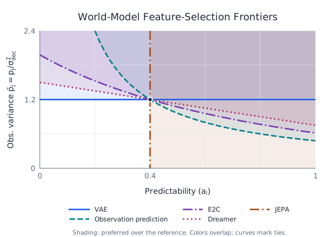
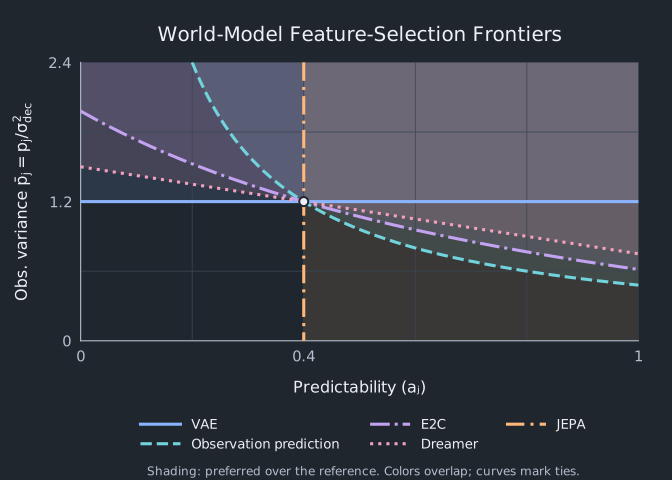
The boundaries mirror the scores: VAE ranks modes only by variance, JEPA only by predictability, while observation prediction, E2C, and Dreamer trade off the two.
To see how the methods differ visually, consider three fixed circles with the same pixel support and texture basis but different dynamics: one varies strongly and unpredictably, one has intermediate variance and high predictability, and one varies least but is the most predictable. Each Transformer must compress the full scene into a one-dimensional latent representation, so we can see which circle each objective prioritizes.
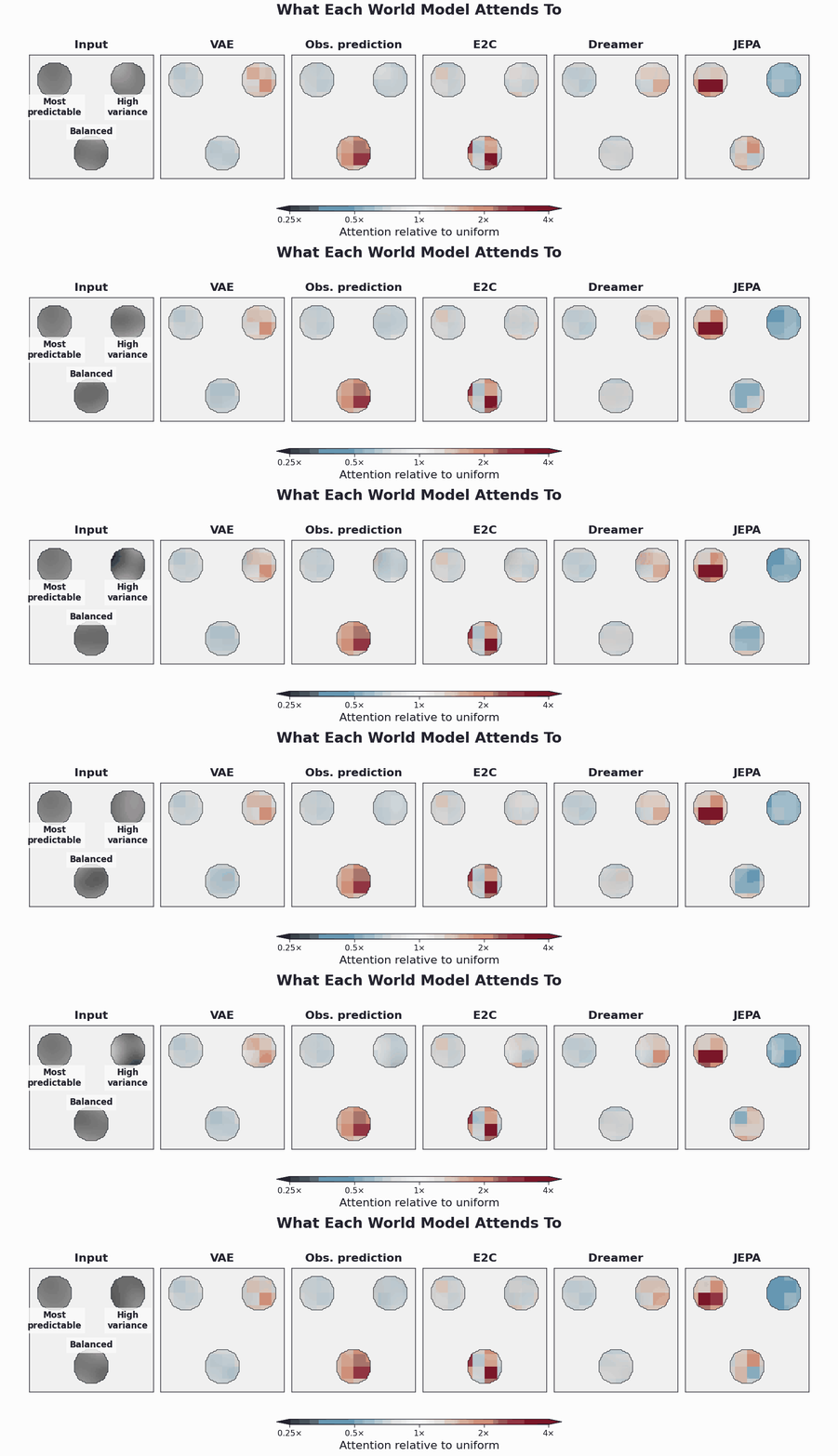
The pattern follows the spectral scores. The VAE focuses on the high-variance mode. Observation prediction focuses on the balanced mode, which has the largest predictable variance \(p_j a_j\). JEPA focuses on the most predictable mode. E2C and Dreamer fall between these extremes.
Stress Test: A Predictable Nuisance Token Can Break LeWorldModel (JEPA)
The scores also suggest objective-specific failure modes that we can test directly. We saw above that JEPA favors slow, predictable features. Here we exploit this preference by adding a task-irrelevant patch that is stable over time and therefore easy to predict, and test whether it can distract the representation from the task. The code for this experiment is available in jepa-stable-token-failure.
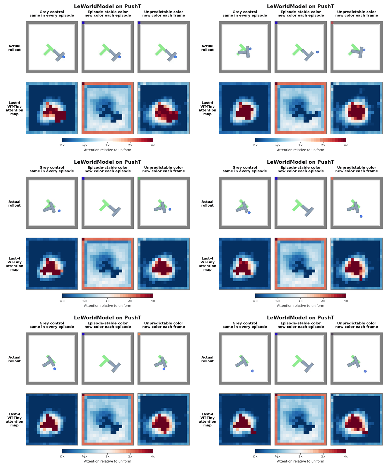
We place the original \(224\times224\) scene inside a \(252\times252\) grey canvas and add one \(14\times14\) colored patch in the top-left corner. The patch occupies exactly one of the model’s 324 image tokens (\(0.31\%\) of the input) and does not alter any task pixel. We train separate models under three conditions: in the grey control, the patch stays grey; with stable color, a random RGB color is sampled once per episode and kept fixed; with unpredictable color, a fresh color is sampled at every model frame. The two colored conditions have the same marginal color distribution. Only temporal predictability changes.
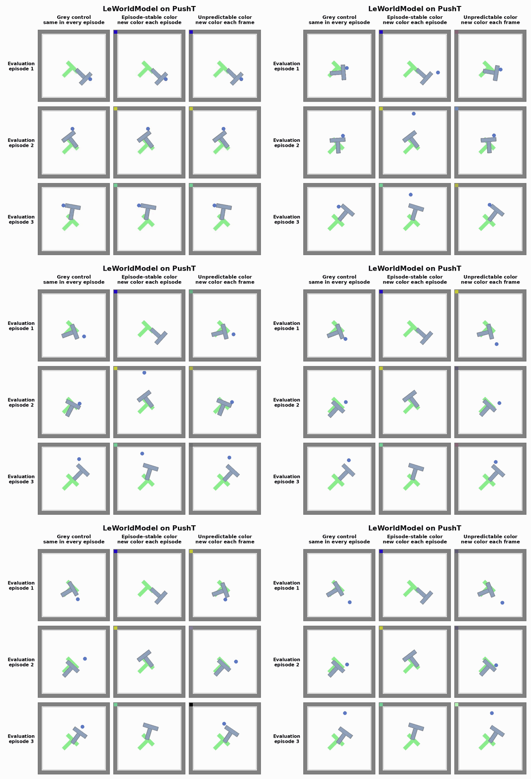
Across ten paired training seeds, this single predictable token nearly destroys planning: success drops from \(79.0\%\) for the grey control to \(1.1\%\) with stable color. Making the same nuisance unpredictable restores success to \(67.7\%\).
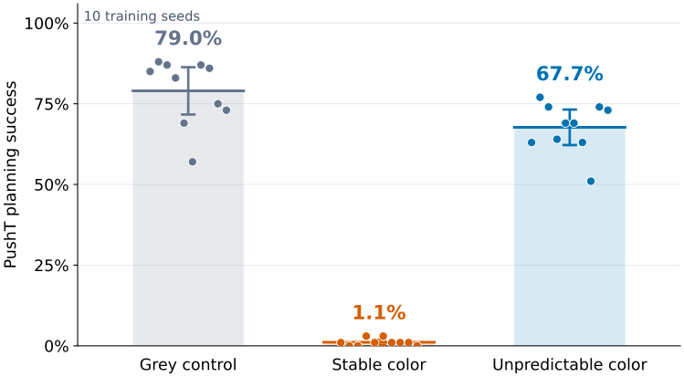
This behavior is exactly what the JEPA objective encourages. The grey patch has no dataset-level variation, so it cannot help satisfy the non-collapse regularizer. The stable colored patch, by contrast, varies across episodes while remaining almost perfectly predictable within each one, making it an attractive feature for the objective. Making the color unpredictable preserves the same marginal variation while removing this temporal shortcut.
The attention maps are consistent with this mechanism. With stable color, attention concentrates on the nuisance token and away from the task. Once the token becomes unpredictable, attention shifts back toward the task-relevant parts of the scene.
Here we expose a JEPA-specific failure mode, but the mode-selection scores can be used to construct a different stress test for each objective. For example, a VAE could fail if a task-irrelevant mode has very high variance and is therefore selected instead of more useful features.
No Free Lunch for World Models
More generally, whether an objective’s preferred features are useful depends on the modality and downstream task. For prediction-based objectives, it also depends on the prediction horizon: a feature that is predictable one step ahead may become unpredictable over longer horizons. Changing the horizon therefore changes which features the objective favors.
Molecular kinetics is a good example. The goal is often to identify the slow collective processes governing transitions between long-lived states rather than reconstruct every instantaneous fluctuation. VAMP
But predictability is not always useful. In speech, for example, speaker identity can stay stable while the phonetic content changes quickly.
More generally, a predictable feature may be persistent, action-driven, or simply a stable nuisance variable. The right feature-selection rule depends on what the downstream task actually requires. Reconstruction favors what varies; latent prediction favors what can be predicted at the chosen horizon
Cite This Post
If you find this post useful, please consider citing it as:
Van Assel, Hugues (2026). Feature Selection in World Models: A Spectral View. October 2. https://huguesva.github.io/blog/2026/world-models/.
@misc{vanassel2026spectral,
  author = {Van Assel, Hugues},
  title  = {Feature Selection in World Models: A Spectral View},
  year   = {2026},
  month  = oct,
  url    = {https://huguesva.github.io/blog/2026/world-models/},
  note   = {Blog post; research-note PDF available at the same URL}
}