Joint-Embedding vs Reconstruction: When Should You Use Each?
A theoretical analysis revealing when joint-embedding methods outperform reconstruction-based SSL, and vice versa.
This blog post presents the key findings from our NeurIPS 2025 paper on comparing two fundamental paradigms in Self-Supervised Learning (SSL): reconstruction-based and joint-embedding methods.
Introduction: Two Paradigms of SSL
Self-Supervised Learning has emerged as a powerful alternative to supervised learning, moving away from specialized labels toward specifying which variations should be disregarded. Two primary families of methods have emerged to learn representations using this principle:
Reconstruction-Based Approaches
Reconstruction-based approaches train models by augmenting an input signal (e.g., adding noise or masking) and then training the model to restore the original input. This process encourages the model to learn meaningful internal representations of the data’s underlying structure. However, because the learning signal arises from minimizing reconstruction error in the input space, the model is naturally steered toward subspaces that explain the majority of the input’s variance.
In language, reconstruction-based learning is highly effective because textual tokens represent compact, semantically meaningful units. Predicting a missing token provides a learning signal that operates directly in semantic space.
In vision, however, variance-explaining features often emphasize aspects that are statistically dominant but semantically shallow. Pixel-level reconstruction objectives tend to drive models toward capturing local statistics and textures rather than higher-order structures and object-level relationships.
Joint-Embedding Approaches
Joint-embedding methods operate entirely in latent space. Their objective is to produce similar representations for different augmented views of the same input while ensuring that representations of distinct samples remain dissimilar. This separation can be enforced explicitly through a contrastive loss, or implicitly via architectural mechanisms such as self-distillation, stop-gradient operations, or predictor heads.
Unlike reconstruction-based approaches, joint-embedding methods do not predict in the input space and are therefore less biased toward capturing high-variance components of the signal. Empirically, joint-embedding frameworks have shown strong performance across domains where the input signal is high-dimensional and semantically diffuse, including histopathology, Earth observation, and video representation learning.
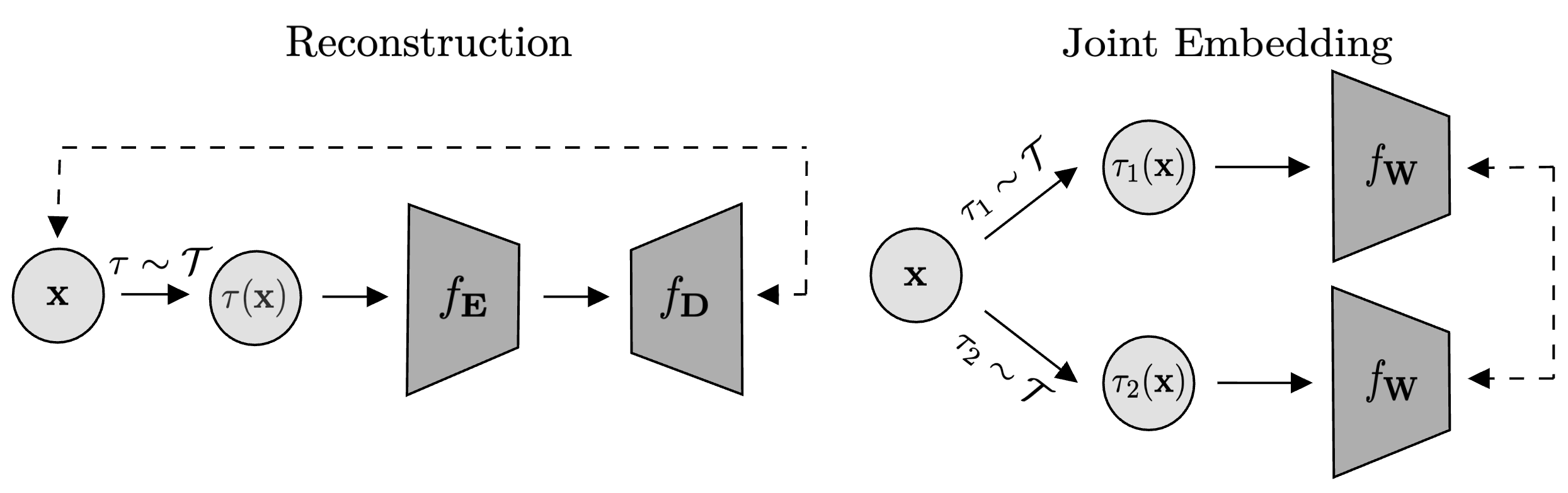
Figure 1: Two self-supervised learning paradigms. Left: Reconstruction approach trains an encoder $f_{\mathbf{E}}$ and decoder $f_{\mathbf{D}}$ to recover $\mathbf{x}$ from augmented view $\tau(\mathbf{x})$. Right: Joint-embedding approach maps two independent augmentations $\tau_1(\mathbf{x})$ and $\tau_2(\mathbf{x})$ to nearby representations via $f_{\mathbf{W}}$.
The Two Main Problems and Their Solutions
Consider \(n\) samples \(\mathbf{X} = (\mathbf{x}_1, \dots, \mathbf{x}_n)^\top \in \mathbb{R}^{n \times d}\) and a data augmentation distribution \(\mathcal{T}\) defined over transformations \(\tau: \mathbb{R}^d \rightarrow \mathbb{R}^d\). For analytical tractability, we focus on linear models: \(f_{\mathbf{E}}: \mathbf{x} \mapsto \mathbf{E} \mathbf{x}\), \(f_{\mathbf{D}}: \mathbf{z} \mapsto \mathbf{D} \mathbf{z}\), and \(f_{\mathbf{W}}: \mathbf{x} \mapsto \mathbf{W} \mathbf{x}\).
Problem 1: Reconstruction-Based SSL
The reconstruction problem is formulated as:
\[\begin{align}\tag{SSL-RC}\label{eq:reconstruction} \min_{\mathbf{E}, \mathbf{D}} \quad \frac{1}{n} \sum_{i=1}^{n} \mathbb{E}_{\tau \sim \mathcal{T}} \left[ \| \mathbf{x}_i - f_\mathbf{D}(f_\mathbf{E}(\tau(\mathbf{x}_i))) \|_2^2 \right] \end{align}\]where \(f_{\mathbf{E}}\) and \(f_{\mathbf{D}}\) are encoder and decoder functions. Each data sample is augmented, encoded, and decoded, with the objective to minimize reconstruction error. This methodology is analogous to Denoising Auto-Encoders and Masked Auto-Encoders (MAE).
Closed-Form Solution for Reconstruction
Theorem 1 (Reconstruction-Based SSL). Let \(\overline{\mathbf{x}}_i := \mathbb{E}_{\tau \sim \mathcal{T}}[\tau(\mathbf{x}_i)]\) denote the expected augmented sample and \(\overline{\mathbf{X}} := (\overline{\mathbf{x}}_1, \dots, \overline{\mathbf{x}}_n)^\top\). Define the covariance of augmented samples:
\[\mathbf{\Sigma} := \frac{1}{n} \sum_{i} \mathbb{E}_{\tau \sim \mathcal{T}} \left[ \tau(\mathbf{x}_i) \tau(\mathbf{x}_i)^\top\right] - \mathbb{E}_{\tau \sim \mathcal{T}} \left[\tau(\mathbf{x}_i) \right] \mathbb{E}_{\tau \sim \mathcal{T}} \left[\tau(\mathbf{x}_i) \right]^\top\]Assume that \(\frac{1}{n} \overline{\mathbf{X}}^\top \overline{\mathbf{X}} + \mathbf{\Sigma}\) is positive definite. Consider the singular value decomposition:
\[\begin{align} \frac{1}{n} \mathbf{X}^\top \overline{\mathbf{X}} \left(\frac{1}{n} \overline{\mathbf{X}}^\top \overline{\mathbf{X}} + \mathbf{\Sigma} \right)^{-\frac{1}{2}} = \mathbf{R} \mathbf{\Phi} \mathbf{P}^\top \end{align}\]where \(\mathbf{R} \in \mathbb{R}^{d \times d}\) and \(\mathbf{P} \in \mathbb{R}^{d \times d}\) are orthogonal and \(\mathbf{\Phi} := \mathrm{diag}(\phi_1, \dots, \phi_d)\) with \(\phi_1 \geq \dots \geq \phi_d \geq 0\).
Solutions of the reconstruction problem \eqref{eq:reconstruction} take the form:
\[\begin{align} \mathbf{E}^\star = \mathbf{T} \mathbf{P}_k^\top \left(\frac{1}{n} \overline{\mathbf{X}}^\top \overline{\mathbf{X}} + \mathbf{\Sigma} \right)^{-\frac{1}{2}} \quad \text{and} \quad \mathbf{D}^\star = \mathbf{R}_k \mathbf{\Phi}_k \mathbf{T}^{-1} \end{align}\]where \(\mathbf{T}\) is any invertible matrix in \(\mathbb{R}^{k \times k}\), \(\mathbf{P}_k\) and \(\mathbf{R}_k\) are the first \(k\) columns of \(\mathbf{P}\) and \(\mathbf{R}\), and \(\mathbf{\Phi}_k = \mathrm{diag}(\phi_1, \dots, \phi_k)\).
Problem 2: Joint-Embedding-Based SSL
The joint-embedding problem is formulated as:
\[\begin{equation}\tag{SSL-JE}\label{eq:ssl} \begin{aligned} \min_{\mathbf{W}} \quad & \frac{1}{n} \sum_{i=1}^{n} \mathbb{E}_{\tau_1, \tau_2 \sim \mathcal{T}} \left[ \| f_\mathbf{W}(\tau_1(\mathbf{x}_i)) - f_\mathbf{W}(\tau_2(\mathbf{x}_i)) \|^2_2 \right] \\ \text{subject to} \quad & \frac{1}{n} \sum_{i=1}^{n} \mathbb{E}_{\tau \sim \mathcal{T}} \left[ f_\mathbf{W}(\tau(\mathbf{x}_i)) f_\mathbf{W}(\tau(\mathbf{x}_i))^\top\right] = \mathbf{I}_k \end{aligned} \end{equation}\]where \(f_{\mathbf{W}}\) is the SSL model. The objective represents the invariance term ensuring consistency between augmented views, while the constraint enforces orthonormality, preventing collapse. This formulation closely resembles methods like SimCLR, VICReg, BYOL, and DINO.
Closed-Form Solution for Joint-Embedding
Theorem 2 (Joint-Embedding-Based SSL). Let \(\mathbf{S} := \frac{1}{n} \sum_{i} \mathbb{E}_{\tau \sim \mathcal{T}} \left[ \tau(\mathbf{x}_i) \tau(\mathbf{x}_i)^\top\right]\) and \(\mathbf{G} := \frac{1}{n} \sum_{i} \mathbb{E}_{\tau \sim \mathcal{T}} \left[ \tau(\mathbf{x}_i)\right] \mathbb{E}_{\tau \sim \mathcal{T}} \left[ \tau(\mathbf{x}_i)\right]^\top\).
Assume that \(\mathbf{S}\) is positive definite. Consider the eigendecomposition:
\[\begin{align} \mathbf{S}^{-\frac{1}{2}} \mathbf{G} \mathbf{S}^{-\frac{1}{2}} = \mathbf{Q} \mathbf{\Omega} \mathbf{Q}^\top \end{align}\]where \(\mathbf{\Omega} = \mathrm{diag}(\omega_1, \dots, \omega_d)\) with \(\omega_1 \geq \dots \geq \omega_d\).
Solutions of the joint-embedding problem \eqref{eq:ssl} take the form:
\[\begin{align} \mathbf{W}^\star = \mathbf{U} \mathbf{Q}_k^\top \mathbf{S}^{-\frac{1}{2}} \end{align}\]where \(\mathbf{Q}_k = (\mathbf{q}_1, \dots, \mathbf{q}_k)\) and \(\mathbf{U}\) is any orthogonal matrix of size \(k \times k\).
These closed-form solutions are directly parameterized by the augmentation structure, enabling us to analyze precisely how augmentations impact learned representations.
Key Findings: Augmentation Alignment Requirements
Using these closed-form solutions, we uncover fundamental differences between the two paradigms. We model data as having \(k\) important signal components and \(d-k\) pure noise components (irrelevant features that SSL should be invariant to). Optimal performance is achieved when the learned representations discard these irrelevant features and retain only the important, meaningful signal components.
We introduce a parameter \(\alpha \geq 0\) that controls the alignment between the irrelevant features and the augmentations. Our main theoretical results reveal:
Finding 1: SSL Requires Aligned Augmentations
Unlike supervised learning, both SSL paradigms require aligned augmentations to achieve optimal performance, even with infinite samples. Simply increasing the sample size cannot overcome misalignment between augmentations and noise.
- Augmentations are well aligned with noise ($\alpha$ large), or
- Sample size is large ($n \to \infty$), regardless of alignment.
- Augmentations are well aligned with noise ($\alpha$ large), or
- Sample size is large ($n \to \infty$) AND alignment satisfies $\alpha > \alpha_{\text{threshold}}$.
This critical difference underscores that carefully designed augmentations are essential in SSL.
Finding 2: Joint-Embedding vs Reconstruction Comparison
Having established that SSL requires aligned augmentations, we now compare the two SSL paradigms. Our second major finding reveals when to prefer each paradigm. Recall that both methods require the alignment parameter $\alpha$ to exceed a certain threshold to achieve optimal performance. Crucially, these thresholds differ between the two paradigms:
- Reconstruction has threshold $\alpha_{\text{RC}}$
- Joint-embedding has threshold $\alpha_{\text{JE}}$
These thresholds depend on noise magnitude, augmentation quality, and data characteristics. A smaller threshold is preferable as it succeeds in more scenarios: since we don’t know noise characteristics in advance, lower alignment requirements mean greater robustness.
Our analysis reveals:
→ Reconstruction is preferable
→ Joint-embedding is preferable
Interpretation
Reconstruction methods prioritize high-variance components: with low-magnitude noise, important features dominate naturally. In contrast, joint-embedding methods operate in latent space, bypassing the need to reconstruct noisy components. With high-magnitude noise, they require less alignment because they avoid reconstructing irrelevant features.
Since data from physical world measurements (images, sounds, sensor recordings) often contain high-magnitude irrelevant features (backgrounds, experimental artifacts), joint-embedding is typically more robust in practice. Our experiments on ImageNet-1k confirm this: joint-embedding methods like DINO and BYOL are considerably more robust to severe data corruption than reconstruction-based methods like MAE.
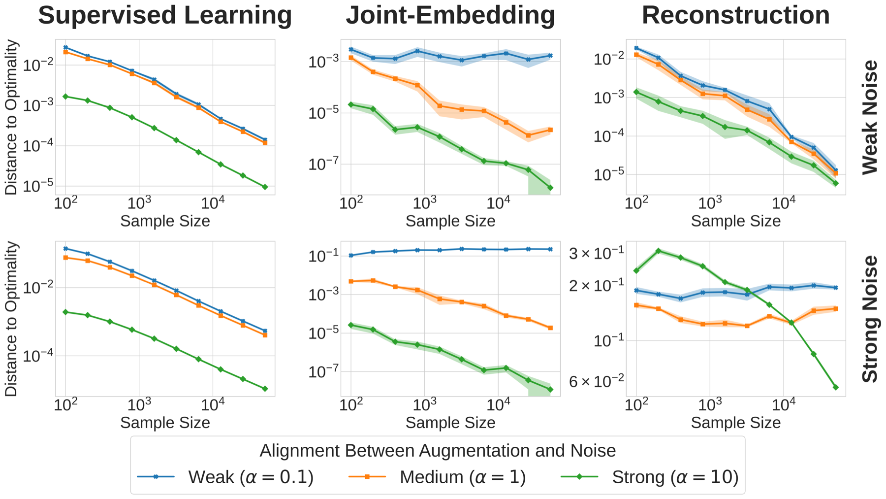
Figure 2: Validation on linear models with MNIST corrupted by synthetic Gaussian noise. Each subplot shows how performance varies with sample size $n$ (x-axis) and augmentation alignment $\alpha$ (different lines). Left: Supervised learning achieves optimal performance with either large $n$ or large $\alpha$, regardless of noise magnitude. Middle: Joint-embedding requires minimal alignment but remains robust even with strong noise. Right: Reconstruction is robust to augmentation choice under weak noise but degrades under strong noise.
Practical Takeaway
- Use Reconstruction when irrelevant features have low magnitude and you have limited knowledge about effective augmentations.
- Use Joint-Embedding when irrelevant features are non-negligible (common in physical world measurements) or when effective augmentations can be identified.
For more technical details, proofs, and comprehensive experimental results, please refer to our full paper.
Citation
If you found this work useful, please cite our NeurIPS 2025 paper:
@inproceedings{vanassel2025je,
  title={Joint-Embedding vs Reconstruction: Provable Benefits of Latent Space Prediction for Self-Supervised Learning},
  author={Van Assel, Hugues and Ibrahim, Mark and Biancalani, Tommaso and Regev, Aviv and Balestriero, Randall},
  booktitle={Advances in Neural Information Processing Systems},
  year={2025}
}